
Creating a balanced investment portfolio with skfolio in Python
Nothing in this article is financial advice. I am not qualified to give financial advice. This is simply an educational article showing one way in which a portfolio could be balanced. No fitness for any purpose is expressed or implied.
Motivation
At the start of the tax year, it’s a natural time for those of us lucky enough to have savings to have a think about how they are invested. Recent turmoil in world equity markets makes this particularly relevant.
Like most retail investors, I think I’m better at choosing where to put my money than I actually am. The Dunning–Kruger effect is in full force, and I like to choose my own investments.
However, I do understand the need to spread risk by having a balanced portfolio. Being a Python developer, it is natural for me to wish to use Python to help me achieve this. This article highlights a reasonable approach that I am considering.
I shall present various code snippets throughout this post, but the full listing (repeating those snippets in context) is at the end.
Python libraries
We’ll be using several Python libraries, together with a simple Python script, to construct balanced investment portfolio.
I recommend using poetry for dependency management, in which case you can
set things up in an empty directory by running:
poetry init(and accepting all the defaults)poetry shellpoetry add skfoliopoetry add yfinancepoetry add matplotlib
Let’s have a quick look at the specific third-part libraries we’ll be using.
skfolio
skfolio, so called because it is built on top of scikit-learn / sklearn, will be doing most of the heavy lifting. It is a library specifically for portfolio optimisation, and has only been around since December 2023.
skfolio is essentially a toolkit for trying and comparing various portfolio theory models. It is a very powerful collection of tools, so we will only be touching on the basics of the functionality it offers in this article. Nevertheless, we will see how simple it can be to build a plausible investment portfolio that attempts to maximise returns and minimise risk.
yfinance
yfinance is a library for downloading financial data from Yahoo! Finance.
This is a very convenient way to get free historical data, as long as you need only daily prices.
Matplotlib
Matplotlib is the standard charting library familiar to most Python users.
We will use it to draw a custom chart of the matrix of correlations between the assets.
Declaring an asset universe
A significant task is defining the total set of assets – shares, bonds, exchange-traded funds (ETFs), etc. – we might consider investing in.
This will depend partly on what the broker makes available, and partly on personal preference (for example, you might choose not to consider equities in certain types of business, or sectors that you think are overvalued).
For the purpose of this article, I’ll choose a small selection of possible investments across equities, bonds and commodities. For using this code in practice I will expand this asset universe considerably: essentially, the more options the better. There are tools in skfolio for filtering down a large asset universe into a smaller one, for example by automatically discarding highly correlated assets, but that is outside the scope of this post.
Choosing the list of potential investments is a non-trivial task. We need to include the symbol used by Yahoo! Finance, which won’t necessarily match the one your broker provides. Generally some web searching is necessary, as well as making sure that the latest prices match up between your broker and Yahoo!
Here is a simple asset universe for us to get started with. Don’t draw any conclusions from this choice; I’m certainly not making any claims about how good or bad it would be to invest in any of these, but they do represent some variety. For practical purposes, you’d choose a much larger pool of potential investments to work with.
ASSETS = [
    # individual companies
    {
        "symbol": "TW.L",
        "name": "Taylor Wimpey",
        "groups": ["uk", "equity"],
        "management_fee": 0.0,
    },
    {
        "symbol": "NG.L",
        "name": "National Grid",
        "groups": ["uk", "equity"],
        "management_fee": 0.0,
    },
    {
        "symbol": "LLOY.L",
        "name": "Lloyds Bank",
        "groups": ["uk", "equity"],
        "management_fee": 0.0,
    },
    {
        "symbol": "BARC.L",
        "name": "Barclays",
        "groups": ["uk", "equity"],
        "management_fee": 0.0,
    },
    {
        "symbol": "MSFT",
        "name": "Microsoft",
        "groups": ["us", "equity", "tech"],
        "management_fee": 0.0,
    },
    # commodities
    {
        "symbol": "GBSS.L",
        "name": "Gold Bullion Securities",
        "groups": ["-", "commodity"],
        "management_fee": 0.4,
    },
    {
        "symbol": "BCOG.L",
        "name": "L&G All Commodities UCITS ETF",
        "groups": ["-", "commodity"],
        "management_fee": 0.02,
    },
    # bonds
    {
        "symbol": "0P0000KM23.L",
        "name": "Vanguard Global Bond Index Fund",
        "groups": ["world", "bonds"],
        "management_fee": 0.15,
    },
    {
        "symbol": "0P0000XBPM.L",
        "name": "Invesco Corporate Bond Fund (UK) Z (Acc)",
        "groups": ["uk", "bonds"],
        "management_fee": 0.5,
    },
]
Notes:
-
This dictionary format is just a convenient grouping of information for later manipulation.
-
The symbol has to match the symbol used by Yahoo! Finance. We use this to download the historic data for the asset.
-
The name doesn’t need to match Yahoo! Finance. It can be whatever makes sense to you.
-
The groups can be any labels that make sense to you. These will be useful for setting constraints (see the next section). Each group needs to have its entries in the same order (here we have used country, asset class and sub-class). It’s fine to omit entries (i.e. I’ve only marked up the
techsub-class); anything else will be automatically treated asNone. -
The management fee is given as an annual percentage. skfolio expects these to be fractions in the same granularity as the data (i.e. daily), so we’ll convert them later.
Setting constraints
One particularly handy feature of skfolio is how you can describe any hard constraints you want to impose on the portfolio as a set of readable strings.
LINEAR_CONSTRAINTS = [
    "tech <= 0.2",
    "uk >= 0.5",
    "us <= 0.1",
    "equity <= 0.7",
    "bonds >= 0.3",
    "commodity <= 0.3",
]
Here we’re imposing the following constraints:
- tech investments (anything with “tech” in its
groups) must constitute at most 20% of the portfolio. - at least 50% of the portfolio must be UK based
- at most 10% of the portfolio may be US based
- at most 70% of the portfolio may be invested in equities
- at least 30% of the portfolio must be invested in bonds
- at most 30% of the portfolio may be invested in commodities
You can also, if you wish, build up more complex conditions, such as uk >= us * 1.5
if you wanted at least one and a half times as much invested in the UK as in the US.
Note that we will also separately use this constraint to prevent more than 20% of the portfolio being invested in any one thing:
MAX_PROPORTION_IN_ONE_ASSET = 0.2
Optimising a portfolio with skfolio
There’s various glue code needed to fetch and transform the data, but let’s concentrate on the most interesting part… feeding the data into skfolio:
X = prices_to_returns(prices)                                         ①
X_train, X_test = train_test_split(X, test_size=0.33, shuffle=False)  ②

model = MeanRisk(                                                     ③
    risk_free_rate=RISK_FREE_RATE / TRADING_DAYS_PER_YEAR,
    objective_function=ObjectiveFunction.MAXIMIZE_RATIO,              ④
    risk_measure=RiskMeasure.VARIANCE,                                ⑤
    min_weights=0.0,
    max_weights=MAX_PROPORTION_IN_ONE_ASSET,
    groups=groups,
    linear_constraints=LINEAR_CONSTRAINTS,
    management_fees=management_fees,
)
model.fit(X_train)

portfolio = model.predict(X_test)
It’s impressive how such a small amount of code is needed to achieve the bulk of what we need for creating a balanced portfolio of investments.
Let’s highlight some important parts:
-
① We convert from raw (closing) prices to linear daily returns: \(\left( \frac{S_t}{S_{t-1}} - 1 \right)\).
-
② Split the historical data into ⅔ training and ⅓ test data. We’re not shuffling, so we’ll be training on old data and testing against more recent data.
-
③ Use the Mean-Risk Optimization estimator, which is a flexible, general-purpose optimiser.
-
④ Use the
MAXIMIZE_RATIOobjective function, which tries to maximise the Sharpe ratio of the portfolio. -
⑤ We want the lowest variance portfolio that can achieve the high Sharpe ratio we find. Ideally we’d like a straight line going up, with no variance at all!
So, this set-up will try to maximize the Sharpe ratio subject to the constraints we set up, and find the portfolio make-up that minimises the variance to get there.
Output
As mentioned before, the full code is at the end of this article. But before we get to that, let’s take a look at the output it generates.
Historical price data
The first thing the script generates is a chart of the historic prices loaded from Yahoo! Finance.
Look out for any missing data or sudden jumps in price. (These happen more
than you would expect because sometimes there’s a sudden switch in reporting
between pounds and pence for UK assets. We set repair=True in the call to
yf.download(), which tries to repair these automatically, but it doesn’t
always get it right.)
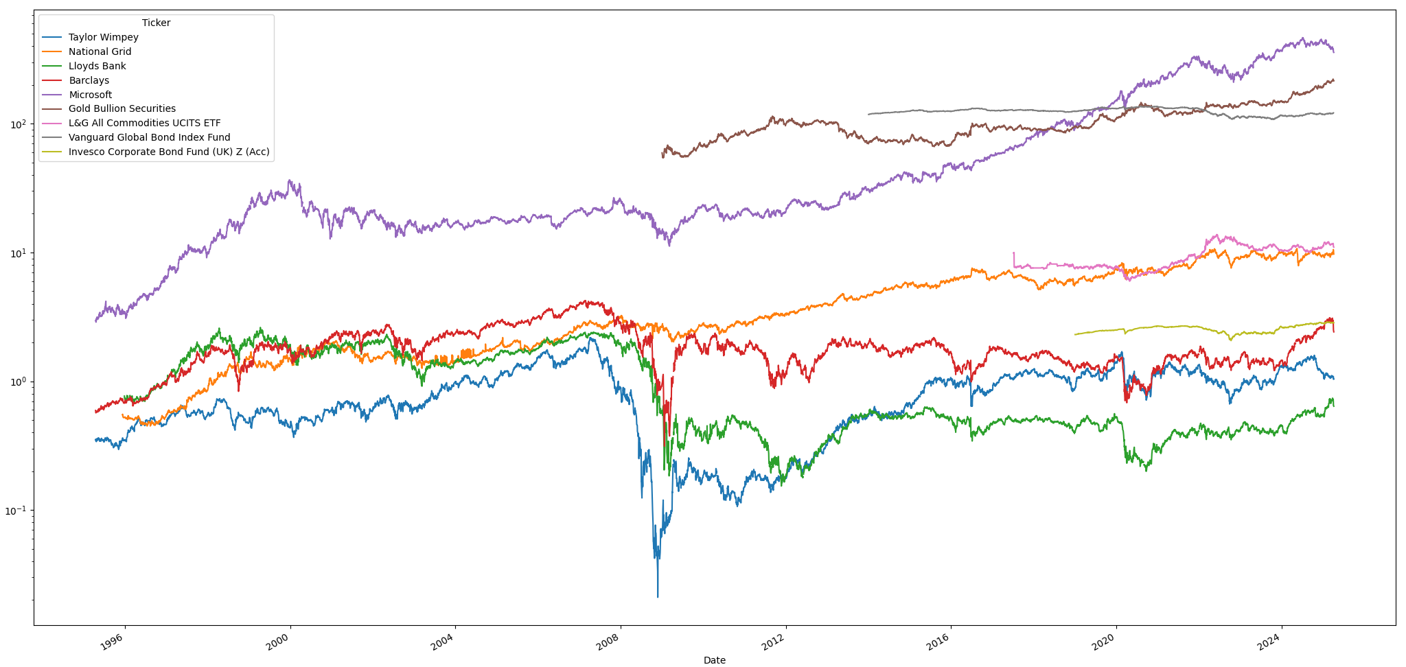
Note that the Y-axis is logarithmic, which makes it easy to see all the asserts with their very different prices on the same chart.
Note also the clear effect of the 2008 market crash, and how some assets were impacted more than others. I wanted enough historic data so that the portfolio takes bad times into account as well as good.
Correlation matrix
The next window shown by the script is a (symmetric) correlation matrix, which shows for each asset how correlated it is with the others.
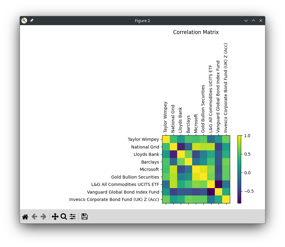
A high correlation (i.e. assets whose prices tend to move in the same direction) is shown in green or yellow. Every asset’s correlation with itself is 1.0, so the leading diagonal of the matrix is bright yellow.
An inverse correlation (i.e. assets whose prices tend to move in opposite directions) is shown in blue.
The third row, for Lloyds Bank, is a good example. Lloyds Bank shares are strongly inversely correlated with shares in the National Grid; but they are strongly positively correlated with shares in Barclays, which shouldn’t be too surprising.
Note also how the Vanguard Global Bond Index Fund and the L&G All Commodities UCITS ETF are very strongly inversely correlated.
So, at a very simple level, if all your investments were split across the two banking assets then you would have very low diversification and a high-risk portfolio (although one that would do very well when banking shares do well). Conversely, investing only across bonds and commodities is likely to give you very low risk – and losses in one area are likely to be offset by profits in the other – but at the same time it might be difficult to make a good return.
For my real portfolio I chose a much larger asset universe, and wanted to see a big spread of colours on this chart to give the algorithm plenty of scope for constructing a balanced portfolio.
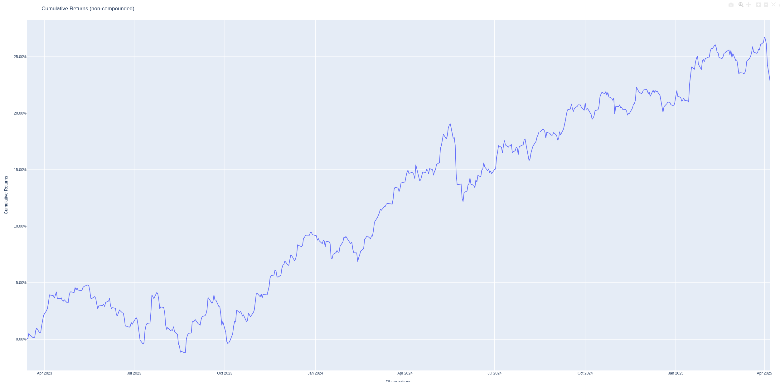
Cumulative returns
The next chart shows what would have happened for the chosen portfolio in the test period.
It’s gone up, which is a good sign ;-)
Here, you’ll notice a tactical error. This chart is supposed to show the performance over the whole test period. But this was 30 years of history in a ⅔ training to ⅓ test split, so you’d expect 10 years of data to be shown.
If you look back at the historical price data, you’ll notice what’s happened.
Not all the data sets go back to the start of the requested period. In
particular, the Ivesco Corporate Bond Fund doesn’t start until 2019. So
skfolio (specifically the call to prices_to_returns) is considering only the
period with data for all assets, so effectively training on 4 years and
testing on 2 instead of the expected training on 20 and testing on 10. I think
that’s reasonable behaviour, but we need to be aware of it. In practice, the
simplest workaround is probably to discard any assets that don’t stretch back
far enough (see DISCARD_SHORT_DATASETS in the script below).
Portfolio composition
The final chart is the meat and potatoes, what we’ve been working towards. This shows which assets the algorithm has chosen, and in which proportions.
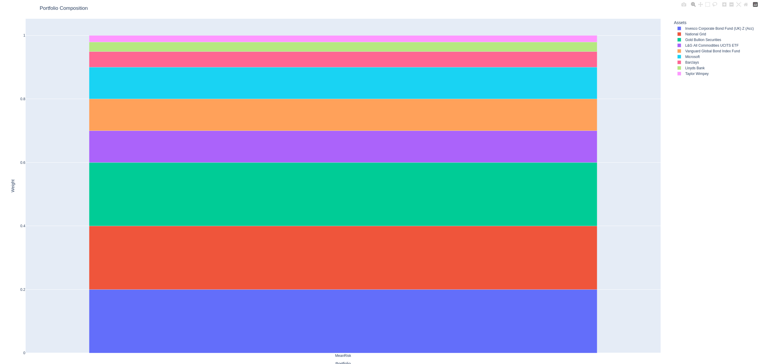
As noted before, this is definitely not investment advice! It’s not even how I plan to invest for myself, it being a cut-down asset universe. But it is indicative of the output you might get.
You can print out the portfolio’s make-up in python, or hover over the chart to see the tooltips.
In this run, the portfolio is comprised as follows:
- 20% Ivesco Corporate Bond Fund
- 20% National Grid
- 20% Gold Bullion Securities
- 10% L&G All Commodities
- 10% Vanguard Global Bond Index Fund
- 10% Microsoft
- 5% Barclays
- 3% Lloyd’s Bank
- 2% Taylor Wimpey
In this case, we had nine assets in our universe and skfolio has allocated some percentage of the portfolio to all of them. That won’t typically be the case for a more realistically large asset universe.
Let’s refer back to the constraints we set:
- tech investments must constitute at most 20% of the portfolio.
- 10% Microsoft <= 20%
- at least 50% of the portfolio must be UK based
- 20% Ivesco + 20% National Grid + 5% Barclays + 3% Lloyd’s + 2% Taylor Wimpey >= 50%
- Since it’s exactly 50% in this case, maybe this is a challenging condition to satisfy.
- at most 10% of the portfolio may be US based
- 10% Microsoft <= 10%
- Again, since it’s exactly on the threshold, it’s likely that more would have been invested in Microsoft if not for this specific constraint.
- at most 70% of the portfolio may be invested in equities
- 20% National Grid + 10% Microsoft + 5% Barclays + 3% Lloyd’s + 2% Taylor Wimpey <= 70%
- at least 30% of the portfolio must be invested in bonds
- 20% Ivesco + 10% Vanguard >= 30%
- Another one on the borderline
- at most 30% of the portfolio may be invested in commodities
- 30% Gold Bullion Securities + 10% L&G Commodities <= 30%
- And, again, right on the borderline.
So, it meets all the constraints that were set and seems like it would have done well if we had invested in such a portfolio for the last couple of years.
As the saying goes, past performance is no guarantee of future success (but it’s all we’ve got).
For those, like me, determined to pick their own investments, skfolio is certainly a more rigorous approach to take over stock picking. I can still control the universe of assets that I am willing to consider investing in, but have some guard rails in terms of imposing sensible constraints on the overall make-up of the portfolio, and some confidence that it will be balanced to maximise returns without undue risk.
Full script
Finally, as promised, here is the full python script I used in this article.
Remember, this is purely illustrative. I won’t even be using it myself in this
form. I would want to add a much larger asset universe to choose from, flip
the DISCARD_SHORT_DATASETS flag to True, and probably take a bit less
history so that fewer assets get discarded, among other changes.
from datetime import date, timedelta, datetime
from pathlib import Path
from pprint import pprint
from skfolio import RiskMeasure
from skfolio.moments import EmpiricalCovariance
from skfolio.moments import EmpiricalMu
from skfolio.optimization import MeanRisk, ObjectiveFunction
from skfolio.portfolio import Portfolio
from skfolio.preprocessing import prices_to_returns
from sklearn.model_selection import train_test_split
from typing import Optional, Union
import matplotlib.pyplot as plt
import numpy as np
import pandas as pd
import yfinance as yf

RISK_FREE_RATE = 0.02
TRADING_DAYS_PER_YEAR = 252
HISTORY_YEARS = 30  # want at least one recession in the training data

# Generally want this to be True, but for this sample script that will discard too many
# assets and the optimiser won't be able to find a solution.
DISCARD_SHORT_DATASETS = False

MAX_PROPORTION_IN_ONE_ASSET = 0.2
LINEAR_CONSTRAINTS = [
    "tech <= 0.2",
    "uk >= 0.5",
    "us <= 0.1",
    "equity <= 0.7",
    "bonds >= 0.3",
    "commodity <= 0.3",
]

# Management fees here are annual percentages, e.g. 1.0 represents a 1% annual fee.
ASSETS = [
    # individual companies
    {
        "symbol": "TW.L",
        "name": "Taylor Wimpey",
        "groups": ["uk", "equity"],
        "management_fee": 0.0,
    },
    {
        "symbol": "NG.L",
        "name": "National Grid",
        "groups": ["uk", "equity"],
        "management_fee": 0.0,
    },
    {
        "symbol": "LLOY.L",
        "name": "Lloyds Bank",
        "groups": ["uk", "equity"],
        "management_fee": 0.0,
    },
    {
        "symbol": "BARC.L",
        "name": "Barclays",
        "groups": ["uk", "equity"],
        "management_fee": 0.0,
    },
    {
        "symbol": "MSFT",
        "name": "Microsoft",
        "groups": ["us", "equity", "tech"],
        "management_fee": 0.0,
    },
    # commodities
    {
        "symbol": "GBSS.L",
        "name": "Gold Bullion Securities",
        "groups": ["-", "commodity"],
        "management_fee": 0.4,
    },
    {
        "symbol": "BCOG.L",
        "name": "L&G All Commodities UCITS ETF",
        "groups": ["-", "commodity"],
        "management_fee": 0.02,
    },
    # bonds
    {
        "symbol": "0P0000KM23.L",
        "name": "Vanguard Global Bond Index Fund",
        "groups": ["world", "bonds"],
        "management_fee": 0.15,
    },
    {
        "symbol": "0P0000XBPM.L",
        "name": "Invesco Corporate Bond Fund (UK) Z (Acc)",
        "groups": ["uk", "bonds"],
        "management_fee": 0.5,
    },
]


def get_adjusted_close(
    ticker: str,
    start_date: Optional[date] = None,
    end_date: Optional[date] = None,
    cache_dir: Union[str, Path] = "cache",
) -> pd.Series:
    if end_date is None:
        end_date = date.today()
    if start_date is None:
        start_date = end_date - timedelta(days=HISTORY_YEARS * 365)

    cache_path = Path(cache_dir)
    cache_path.mkdir(parents=True, exist_ok=True)

    start_str = start_date.isoformat()
    end_str = end_date.isoformat()
    cache_file = cache_path / f"{ticker}_{start_str}_{end_str}.pkl"

    if (
        cache_file.exists()
        and datetime.fromtimestamp(cache_file.stat().st_mtime).date() == date.today()
    ):
        print(f"Reading {ticker} from cache.")
        data = pd.read_pickle(cache_file)
    else:
        print(f"Reading {ticker} from Yahoo Finance.")
        data = yf.download(
            ticker,
            start=start_str,
            end=end_str,
            repair=True,  # automatically cope with 100x switches between pounds and pence
        )
        if data is not None:
            data.to_pickle(cache_file)
        else:
            raise RunTimeError(f"Failed to download data for {ticker}. Stopping.")

    if "Adj Close" in data:
        return data["Adj Close"]
    else:
        return data["Close"]


def optimise(
    prices: pd.DataFrame,
    groups: dict[str, list[str]],
    management_fees: dict[str, float],
) -> None:
    # plot all the price data to check it's sensible
    prices.plot(logy=True)

    if DISCARD_SHORT_DATASETS:
        cols_to_drop = prices.columns[prices.iloc[0].isna()]
        print("Dropping assets where the data doesn't go back far enough:", list(cols_to_drop))
        prices = prices.drop(columns=cols_to_drop)

    X = prices_to_returns(prices)
    X_train, X_test = train_test_split(X, test_size=0.33, shuffle=False)

    model = MeanRisk(
        risk_free_rate=RISK_FREE_RATE / TRADING_DAYS_PER_YEAR,
        objective_function=ObjectiveFunction.MAXIMIZE_RATIO,
        risk_measure=RiskMeasure.VARIANCE,
        min_weights=0.0,
        max_weights=MAX_PROPORTION_IN_ONE_ASSET,
        groups=groups,
        linear_constraints=LINEAR_CONSTRAINTS,
        management_fees=management_fees,
    )
    model.fit(X_train)

    portfolio = model.predict(X_test)
    pprint(portfolio.summary())

    returns = portfolio.plot_cumulative_returns()
    returns.show()

    plot_correlation_matrix(prices.corr(), list(prices))

    composition = portfolio.plot_composition()
    composition.show()


def plot_correlation_matrix(cov: np.ndarray, labels: list[str] = None) -> None:
    fig, ax = plt.subplots(figsize=(8, 6))
    cax = ax.matshow(cov, cmap="viridis")
    fig.colorbar(cax)

    if labels:
        ax.set_xticks(range(len(labels)))
        ax.set_yticks(range(len(labels)))
        ax.set_xticklabels(labels, rotation=90)
        ax.set_yticklabels(labels)

    ax.set_title("Correlation Matrix", pad=20)
    plt.tight_layout()
    plt.show()


if __name__ == "__main__":
    price_series = [
        get_adjusted_close(asset["symbol"]).rename(
            columns={asset["symbol"]: asset["name"]}
        )
        for asset in ASSETS
    ]
    prices = pd.concat(price_series, axis=1)

    for series in prices:
        print(f"Latest price for {series} is {prices[series][-1]}")

    groups = {asset["name"]: asset["groups"] for asset in ASSETS}

    management_fees = {
        asset["name"]: (asset["management_fee"] / 100) / TRADING_DAYS_PER_YEAR
        for asset in ASSETS
    }

    optimise(prices, groups, management_fees)
Edits:
2025-04-09 Removed pointless second constraint for the US from the full code listing.